
The lower-body injury analysis was a very unbalanced dataset containing a small number of injuries with a large set of plays without injuries. The data without injuries functioned as a control group used for classification in a supervised analysis. The initial model used Random Forests, as it produced a very high accuracy. However, the precision was the more important consideration with the imbalanced data, and the neural network model provided a much higher precision than did the ensemble learning.
All instances of the concussion data were incidents with concussions, preventing us from using a supervised model. The best results were achieved with a PCA feature extraction, reducing the features to 3 dimensions, more ideal for visualization. Following the feature extraction, K-Means clustering was used to classify the data into the groups. Both a dendogram and an elbow curve were used to determine the number of cluseters to use. Because of the ambiguity incurred with the feature extraction, we used a Random Forest classifier to determine which features had the strongest association with each of the outputs.
The goal with the initial analysis was to determine whether we could predict whether an injury occurred based on all feautures, such as temperature, turf, weather, etc., excluding the tracking data from the individual players.
Due to the nature of the Injury Dataset being extremely imbalanced, we used the Balanced Random Forest Classifier from the imbalanced learn library. In preparing the data for processing, the positions were encoded in a single column by numbers, as described above, however the plays were encoded with OneHotEncoder, giving us 3 columns for each of the plays.
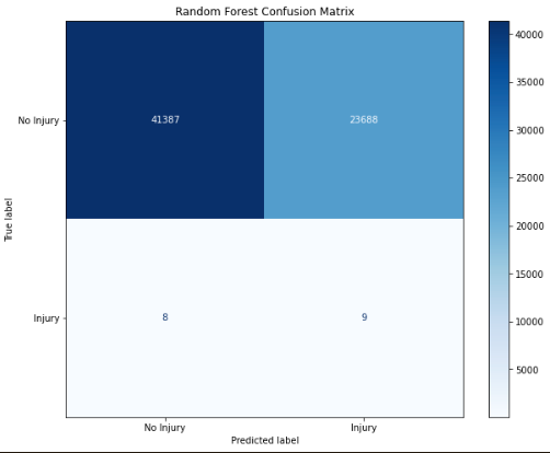
In determining whether an injury occurred, the original model achieved a 58% accuracy and worse precision. We futher analyzed the feature importances.
The original dataset contained 260,000 rows with only 77 injuries. Because of this large difference, we tried several approaches, including Undersampling and SMOTEENN, but ultimately, we just split the data using train_test_split() from the scikit learn library both with and without stratification.
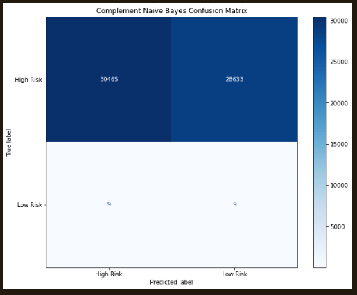
The next analyses utilized a Complement Naive Bayes analysis; this type of Naive Bayes is more suitable for extremely imbalanced datasets. Similar to the Random Forest model, the results only provided a 58% accuracy. Likewise, an EasyEnsemble Boosting algorithm was tested again with similar results. From these analyses, we concluded that additional information would be necessary to further improve our models. The Random Forest and Complement Naive Bayes are shown below:
Futher development of the dataset included the spatial parameters that should gave more predictive capability, indicating the great impact on the potential for injury. Using these data with random sampling the non-injury data were reduced to achieve a 100:1 distribution from the 3000:1 distribution we started with. Once the spatial data were added, this dataset expanded substantially, making a big impact on processing. Each of the Random Forest models was able to predict with 99% accuracy, and few to no false negatives:
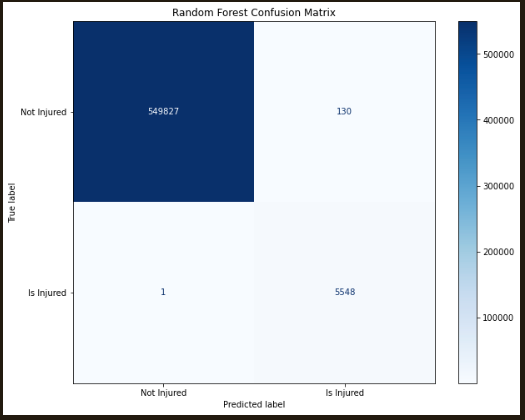
The adaptations from the original model to the final models for the Injury Data was the addition and cleaning of the tracking data. With the addition of the tracking information, the Balanced Random Forest Classifier with 10 estimators provided a 99.96% accuracy, a much higher accuracy than was achieved with the any of the models not including the tracking data. With the addition of the tracking data, the number of rows increased to several thousand. In addition to the 99.97% accuracy, this model yielded under 5 false negatives, and 145 false positives from the dataset including 550,000 true negatives and 5500 true positives.
In the feature analysis, we confirmed that the strongest feature in the feature analysis was the number of days played, closely followed by the temperature, and the time of the play during the game. Other stronger predictors were the player's position and the location along the length of the field.
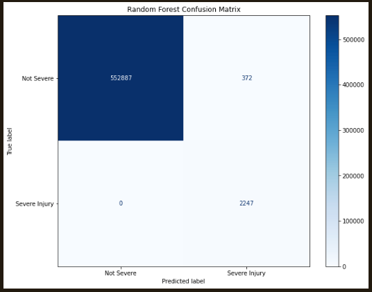
Was the injury severe? The same process as above was followed, yielding a 99.97% accuracy and a lower, 90.35% precision.
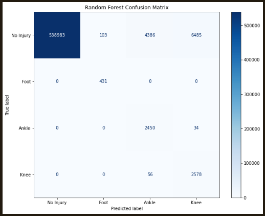
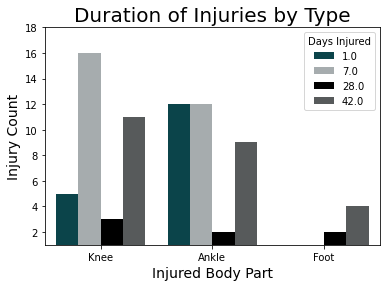
What type of injury was predicted? The overall accuracy of this model with 4 outputs was again 98.59%, but the precision started to really drop:
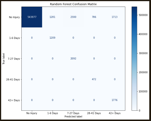
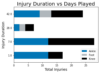
What was the predicted duration of injury? The overall accuracy remains high at 99.77%, but the precision continues to drop:
The Random Forest Classifiers predicting multiple outcomes were more difficult to predict the accuracy and recall specifically, and they were not possible to evaluate like this for the neural network model. These results were summarized in the following table:
| Test | Model | Accuracy | Precision | Recall |
|---|---|---|---|---|
| Is Injured | Random Forest | 0.9995 | 0.9743 | 0.9995 |
| Severe Injury | Random Forest | 0.9998 | 0.9035 | 1.0000 |
| Injured Foot | Random Forest | 0.9860 | 0.7894 | 1.0000 |
| Injured Ankle | Random Forest | 0.9860 | 0.4261 | 0.9823 |
| Injured Knee | Random Forest | 0.9860 | 0.2745 | 0.9799 |
| Duration - Under 1 Week | Random Forest | 0.9977 | 0.6000 | 1.0000 |
| Druation - 1-4 Weeks | Random Forest | 0.9977 | 0.3567 | 0.9995 |
| Duration - 4-6 Weeks | Random Forest | 0.9977 | 0.5612 | 1.0000 |
| Duration - Over 6 Weeks | Random Forest | 0.9977 | 0.6375 | 1.0000 |
In the final model, there were some changes made from the preliminary models:
| Test | Model | Accuracy | Loss | Precision | Recall |
|---|---|---|---|---|---|
| Is Injured | Neural Network | 0.9956 | 0.0127 | 0.9412 | 0.5969 |
| Severe Injury | Neural Network | 0.9997 | 0.0009 | 0.9844 | 0.9533 |
| Injury Type (4-class) | Neural Network | 0.9993 | 0.0016 | 0.9994 | 0.9991 |
| Injured Foot | Neural Network | 0.9998 | 0.0006 | 1.0000 | 0.7703 |
| Injured Ankle | Neural Network | 0.9994 | 0.0023 | 0.9003 | 0.9638 |
| Injured Knee | Neural Network | 0.9995 | 0.0010 | 0.9792 | 0.9115 |
| Injury Duration (5-class) | Neural Network | 0.9994 | 0.0009 | 0.9992 | 0.9994 |
Similar to the Injury Analysis, the tables were merged including the tracking data, creating a very large dataset. In order to perform the clustering analysis, there are several ways to break the data into different clusters. The first approach was using Agglomerative Clustering, which required a size reduction to create a dendogram. The dendogram shows the highest break at two, followed by three clear clusters.
This analysis was performed with 3 clusters prior to breaking up into two sets using train_test_split for feature classification. A Balanced Random Forest Classifier was used with 100 estimators to determine which features have the highest correlation with the different classes. In this case, the highest correlation was the Twist, the difference between the orientation of the player and the direction of movement.

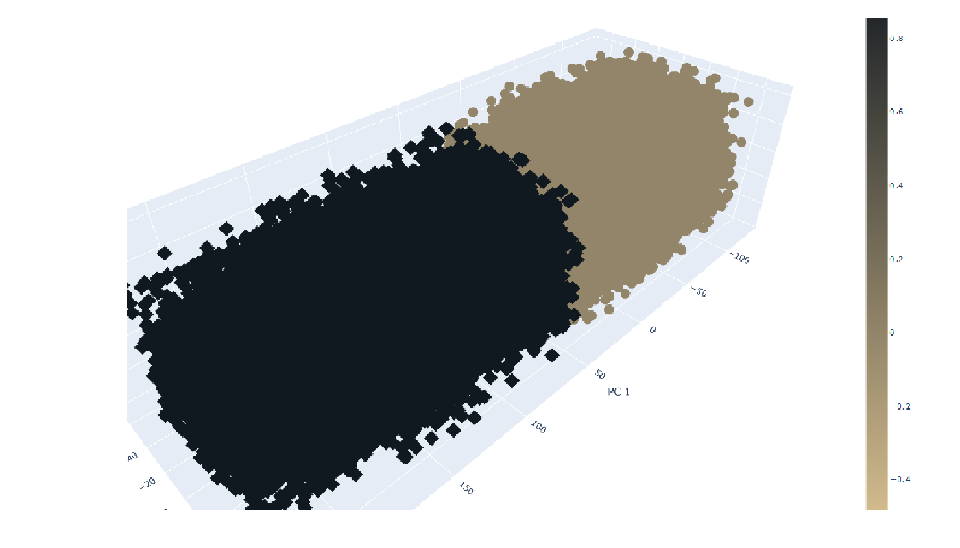
Following the Agglomerative Clustering, we used PCA data extraction to reduce the dimensions to 3 components. Testing for the ideal number of clusters for K-Means analysis, we utilized an elbow curve, where there was a very distinct bend at k=2. The K-Means clustering was performed with 2 clusters. The K-Means analysis was plotted using hvplot as shown below: